
17 Independence Assumptions (Part 2)
17.1 Non-Independence of Housing Market
- Actual story is a bit more complicated: correlations were modeled, using a Gaussian copula
- Basic idea: sample debt payouts from a multivariate Gaussian (with specified correlation structure)
- Issue: payouts don’t follow normal distribution. So apply 1-dimensional transformation to each payout to give it desired distribution shape.
- Big problem: despite correlation in bulk, no tail dependence (extremes in one variable don’t imply extremes in othr)
- Colloquially: conditional on \(X_1\) being in the 99.9th percentile, the probability that \(X_2\) is also in 99.9th percentile is close to zero in the model, but not in reality.
17.1.1 What is a Gaussian Copula?
samples = sample_gaussian(10,0.9)
plt.gca().set_aspect('equal', adjustable = 'box')
plt.scatter(samples[:, 0], samples[:, 1])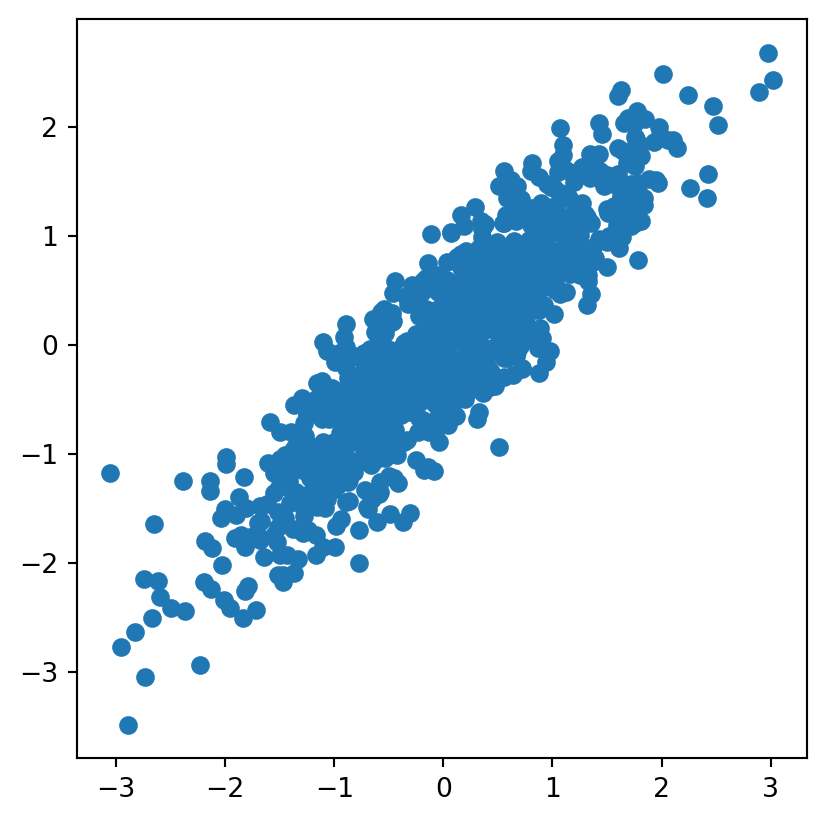
\[ d = 3 \implies \begin{bmatrix} 1 & \rho & \rho \\ \rho & 1 & \rho \\ \rho & \rho & 1 \end{bmatrix} \]
Instead of Gaussian they are Uniform(0, 1) but still have a correlation from the multivariate gaussian.
17.1.2 Transformation
Transform each coordinate to make uniform. How do we transform a gaussian to uniform?
\[\begin{align*} v &\sim \mathcal{N}(0, 1) \\ \Phi(x) &= P[X < x] \\ P[\Phi(v) < t] &= t\quad\forall t\in[0,1] \\ P[v<x] &= \Phi(x) \\ P[\Phi(v) < t] &= \Phi(\Phi^{-1}(t)) = t \end{align*}\]
For the Gaussian so you can see in both cases. They have. Correlation, but the overall shape of the distribution is different.
But. Clearly things are still correlated, which is what I wanted. But what happens if I start looking at just The upper right.
17.2 General copulas
17.2.0.1 Introduction to Copulas
In the realm of statistical modeling, copulas are a powerful tool for understanding and manipulating the dependencies between different variables. They allow us to model the joint distribution of multiple variables by understanding the marginal distribution of each variable independently. A fundamental application of copulas involves transforming a Gaussian distribution into various other types of distributions, such as uniform, Bernoulli, or Student’s \(t\) distributions. This transformation is crucial for tailoring statistical models to better fit the characteristics of real-world data, especially when the Gaussian distribution’s symmetry and light-tailed nature do not adequately capture the underlying phenomena.
17.2.0.2 Transforming Gaussian to Uniform Distribution
The first step in utilizing copulas for distribution transformation is converting a Gaussian distribution into a uniform distribution. This is achieved through the application of the Cumulative Distribution Function (CDF) of the Gaussian distribution to its samples. The CDF maps the samples to a uniform distribution on the interval [0, 1], serving as a bridge to further transformations.
17.2.0.3 Generalizing to Other Distributions
However, the journey doesn’t end with uniform distributions. The real power of copulas lies in their ability to transition from a uniform distribution to virtually any target distribution. This transition is facilitated by the inverse CDF (also known as the quantile function) of the target distribution. By applying the inverse CDF of the target distribution to the uniformly distributed samples, we can mold our data to follow the desired distribution.
17.2.0.4 Case Study: Transition to a Student’s \(t\) Distribution
Let’s consider a scenario where the target distribution is chosen to be a Student’s \(t\) distribution, known for its heavier tails compared to the Gaussian distribution. This choice is motivated by the need to model data that exhibits heavy-tailed behavior, which is common in financial markets, insurance claim sizes, and many natural phenomena.
Suppose we aim to transform our Gaussian samples into a Student’s \(t\) distribution with 3 degrees of freedom, a specific parameter that controls the heaviness of the tails. The process involves two main steps: Gaussians do not model global correlations
17.2.1 Multivariate \(t\) distributions
17.2.1.1 Gaussian Distribution and Its Limitations
The Gaussian distribution is a fundamental tool for describing the distribution of continuous variables. However, it has its limitations, particularly when it comes to modeling phenomena that exhibit multiplicative behavior, such as housing prices. A key limitation is its inability to naturally accommodate percentage-based changes across a dataset. For example, while a Gaussian model can easily describe a scenario where all housing values decrease by a fixed amount, say $5, it struggles to represent situations where values decrease by a percentage, such as 5%.
17.2.1.2 The Log-Normal Distribution and Housing Prices
Housing prices, with their multiplicative fluctuations, are more aptly described by a log-normal distribution. This distribution accounts for the fact that housing prices cannot go below zero and tend to exhibit right-skewed behavior, where a significant number of properties are of average value, but a few can be extremely expensive. The log-normal distribution captures these characteristics by assuming that the logarithm of housing prices follows a normal distribution, thereby accommodating multiplicative changes more naturally than a Gaussian distribution.
17.2.1.3 Transition to the Multivariate Student’s \(t\) Distribution
While the log-normal distribution provides a better fit for housing prices than the Gaussian distribution, it still does not fully capture the complexity of real-world data, especially when considering the correlation between multiple variables or assets. This is where the concept of copulas, and specifically the T-copula, comes into play. A T-copula allows for the modeling of dependencies between multiple variables, offering a way to construct a multivariate distribution that captures the tail dependencies and correlations observed in real-world data.
The multivariate Student’s \(t\) distribution emerges as a powerful tool in this context. Unlike the Gaussian distribution, the Student’s \(t\) distribution has heavier tails, which means it can better model the likelihood of extreme outcomes. This characteristic is particularly useful in financial and economic models, where extreme events, while rare, can have significant impacts.
Transitioning to a General Student’s \(t\) Distribution through Copulas Introduction to Advanced Copula Applications In the exploration of statistical modeling and distribution transformations, we’ve seen how copulas enable the transition from Gaussian distributions to uniform distributions and then to other target distributions like the Student’s \(t\). This process highlights the versatility of copulas in modeling complex data distributions. The final step in this exploration involves moving from a uniform Student’s \(t\)-based copula to a more general Student’s \(t\) distribution, showcasing the full potential of copulas in capturing the intricacies of data behavior.
From Uniform to Target Distribution The foundational principle behind this transformation is the application of the inverse Cumulative Distribution Function (CDF) of the target distribution to uniformly distributed samples. This method, which has been effective in previous transformations, remains our tool for achieving the desired distribution characteristics.
Implementing the Transformation Starting with samples that are uniformly distributed as a result of applying a Student’s \(t\)-based copula, we proceed by applying the inverse CDF of our target distribution. In this context, our aim is to compare the outcomes of transforming these samples into a normal distribution against those obtained directly from a Student’s \(t\) distribution.
17.3 Comparative Analysis: Student’s \(t\) vs. Gaussian Copula
To illustrate this process, consider two sets of samples:
One set obtained from the Student’s \(t\) distribution. Another set derived from a Gaussian copula, both aimed to be transformed into a normal distribution. Upon applying the transformation, we observe the resulting distributions. The comparison reveals that, while there are similarities, notable differences emerge:
- Student’s \(t\) Samples (Blue): These samples, characterized by their heavier tails, indicate a stronger correlation in extreme values (tails) but less so in the central part of the distribution (bulk).
- Gaussian Copula Samples (Orange): In contrast, these samples exhibit a different pattern of correlation, with nuances that distinguish them from the Student’s \(t\) samples.
Observations and Insights The visual comparison of the transformed distributions provides valuable insights:
Tail Behavior: The Student’s \(t\) distribution’s heavier tails are evident, suggesting its suitability for modeling data with potential extreme values.
Correlation Patterns: The differences in correlation between the tails and the bulk of the distributions highlight the importance of choosing the right model based on the specific characteristics of the data.
The final exploration in our journey through statistical transformations using copulas aims to transition from a uniform Student’s \(t\)-based copula to a general Student’s \(t\) distribution. This step represents a sophisticated application of copulas, demonstrating their versatility in statistical modeling and distribution transformation.
17.3.0.1 The Process
The methodology remains consistent with the principles we’ve previously established:
- Starting Point: We begin with uniformly distributed random variables, achieved through the application of a Student’s \(t\)-based copula.
- Transformation: To transition to a target distribution, we employ the inverse Cumulative Distribution Function (CDF) of the target distribution. This approach allows us to mold our uniform distribution into the desired shape and characteristics. #### Application and Comparison In this scenario, the target distribution is chosen to be the normal distribution. This choice facilitates a comparison between:
Samples directly derived from a Student’s \(t\) distribution. Samples transformed from a Gaussian copula to the normal distribution. Observations from the Transformation Upon applying the inverse CDF to achieve the normal distribution, we observe the outcomes:
- Visual Comparison: The distributions of the transformed samples (from both the Student’s \(t\) and the Gaussian copula) are closely aligned, indicating the effectiveness of the transformation process.
- Differences in Correlation: Notably, the Student’s \(t\) samples (represented in blue) exhibit more correlation in the tails and less in the central bulk compared to the Gaussian samples (in orange). This difference highlights the distinct characteristics of the Student’s \(t\) distribution, particularly its heavier tails and the implications for modeling data with extreme values. #### Insights and Implications
- Tail Behavior: The comparison underscores the Student’s \(t\) distribution’s capacity to model heavy-tailed phenomena, a critical attribute for fields dealing with extreme events, such as finance and risk management.
- Model Selection: The subtle differences between the distributions emphasize the importance of selecting the appropriate model based on the data’s characteristics. The choice between a Student’s \(t\) and a Gaussian approach depends on the specific requirements for tail behavior and correlation structure.
17.3.1 Analyzing Mortgage Correlations with Gaussian and Student’s \(t\) Copulas
Understanding the correlation between different financial instruments, such as mortgages, is crucial for risk management and investment strategy. This analysis explores the impact of correlation on the risk profiles of mortgage portfolios using two different copulas: Gaussian and Student’s \(t\). The focus is on how these copulas predict the behavior of portfolio values under varying degrees of correlation.
17.3.1.1 Correlation Assumption
Let’s assume a modest correlation between different mortgages at 0.2. This correlation reflects a realistic scenario where mortgages, while largely independent, can exhibit some degree of synchronicity in their performance due to common underlying factors such as economic conditions or interest rates.
17.3.1.2 Gaussian vs. Student’s \(t\) Copulas
The comparison between Gaussian and Student’s \(t\) copulas reveals significant differences in how they model risk, especially in extreme scenarios:
Gaussian Copula: This model suggests a lower bound on portfolio losses, indicating that the portfolio value is unlikely to drop below 0.6 or 0.5. This optimistic scenario implies a limited risk of severe losses, portraying a relatively stable investment.
Student’s \(t\) Copula: In contrast, the Student’s \(t\) copula presents a more cautious picture, showing that portfolio values could potentially plummet to as low as 0.3. This indicates a higher risk of significant losses, suggesting that the “senior tranche” of the investment could lose nearly half of its value in adverse conditions.
17.3.1.3 Impact of Correlation Variability
Exploring further, let’s consider the effect of adjusting the correlation:
Lower Correlation (e.g., 0.1): With an even lower correlation, the Gaussian copula shows a very concentrated risk profile compared to the Student’s \(t\) copula. This difference highlights how Gaussian models may underestimate the risk of tail events.
Higher Correlation: As the correlation increases, the disparity between the Gaussian and Student’s \(t\) copulas begins to diminish. However, even at high correlation levels, the Student’s \(t\) copula still indicates a non-negligible risk of extreme losses.
17.3.1.4 Conclusions and Implications
This analysis underscores the importance of choosing the appropriate copula model for financial risk assessment. The Gaussian copula, with its assumption of normality and lighter tails, may not fully capture the risk of extreme loss scenarios. On the other hand, the Student’s \(t\) copula, with its heavier tails, offers a more conservative and arguably more realistic assessment of risk, especially in portfolios with low to moderate correlation.
For investors and risk managers, the choice between these copulas can significantly affect the perceived risk profile of mortgage portfolios. The Student’s \(t\) copula’s ability to model more extreme outcomes suggests it may be a more prudent choice for stress testing and risk management purposes, particularly in uncertain economic environments.
This analysis highlights the nuanced trade-offs between different statistical models in financial risk management, emphasizing the need for careful model selection based on the specific characteristics of the investment and the risk tolerance of the stakeholders involved