14  Numerical Methods for Combining Considerations

14.1 Overview

In this section we will formalize some ways we can combine various considerations of numerical and structural uncertainty. We continue with the UK Omicron hospital peak example from the previous lectures.

In the previous section, we covered:

• Numerical sensitivity
• Structural uncertainty
• High-level methods for combining the two together

In this section, we will cover formal methods for combining considerations

• Squiggle (software tool): link to Squiggle documentation
• Graphical method (by hand)

14.2 Squiggle for Numerical Sensitivity

Recall from the previous section our goal of forecasting the number of days until the UK hospital peak using information as of Dec. 21, 2021. We came up with the following table of relevant parameters and 70% confidence intervals for each. Our final formula to combine the parameters to get the number of days until the peak was: \[\log _2\left(N / 2 \mathrm{N}_0\right) \ast \mathrm{t}+\Delta_0+\Delta_1\]

Parameter	Point estimate	Range	Effect on answer
\[ N_0 \]	\[ 0.2 \times 10^6 \]	\[ [0.15, 0.25] \times 10^6 \]	\[ [-0.8, +1.0] \]
\[ N \]	\[ 6.7 \times 10^6 \]	\[ [5, 13] \times 10^6 \]	\[ [-1.0, +2.3] \]
\[ t \]	\[ 2.4 \]	\[ [2.0, 3.3] \]	\[ [-1.6, +3.7] \]
\[ \Delta_0 + \Delta_1 \]	\[ 12 \]	\[ [9, 14] \]	\[ [-3, +2] \]

Suppose we want to go from the error bars on the individual parameters to error bars on our final estimate to produce a 70% confidence interval. We did this heuristically in the last section, but ideally we would model each of the parameters as a distribution and combine their distributions to get a distribution on the final answer. We will now walk through a demo of how to use Squiggle to automatically model the distributions of the parameters and combine them to produce our forecast. You can follow along with the Squiggle demo here.

We begin by inputting the parameters and our formula for how to combine them:

casesSoFar = 150k to 250k
totalCases = 5M to 13M
doublingTime = 2.0 to 3.3
lag = 9 to 14
daysUntilPeak = log(totalCases/(2*casesSoFar))/log(2)*doublingTime + lag

There are a couple improvements we need to make to this:

• By default, Squiggle interprets these ranges as 90% confidence intervals. However, these ranges from last lecture were our 70% confidence intervals. We want to be able to control the confidence level.
• We would prefer to return an actual date, not the number of days until the peak.

We begin with the easier of the three improvements listed above: returning a date. Fortunately, Squiggle provides a nice date library that we can leverage. The first line of the code below adds t days to December 12, 2021 to get the date of our forecasted peak. The lines that follow grab the SampleSet, turn it into a list, get the desired quantiles, and put them into the date function.

getDate(t) = {
  Date.make('2021-12-21') + Duration.fromDays(t)
}
getQuantile(s, q) = {
  quantile(SampleSet.toList(s), q)
}
lower = getDate(getQuantile(daysUntilPeak, 0.15))
upper = getDate(getQuantile(daysUntilPeak, 0.85))

Next we tackle the problem of converting our 90% confidence intervals into 70% confidence intervals. The code below defines a function that allows us to convert our ranges from 90 to 70% confidence. We pre-computed factor using Numpy, and we can change the confidence level by changing factor. Note that the last line of the function is what gets returned.

dist70(low, high) = {
  logmu = (log(high) + log(low))/2
  logwidth = (log(high) - log(low))
  factor = 1.0364333894937898 // ratio between 70% CI and stdev of a normal distribution
  logsigma = logwidth/(2*factor)
  exp(normal(logmu, logsigma))
}

We can us our newly defined dist70 function to re-express our intervals with 70% confidence as follows:

casesSoFar = dist70(150k, 250k) 
totalCases = dist70(5M, 13M)
doublingTime = dist70(2.0, 3.3)
lag = dist70(9, 14)

Following along with the demo, Squiggle indicates on the right sidebar that Jan 08, 2022 to Jan 17, 2022 should be our forecast.

14.3 Squiggle for Structural Uncertainty

We will now see how we can use Squiggle for structural uncertainty. Recall our considerations from the previous lecture:

• Herd immunity: 15% chance of +5 days (28 million vs. 7 million cases)

• Short doubling time: 15% chance of -4 days (1.5 vs. 2.4 day doubling)

• Extended peak: 10% chance of +[0,12] days

You can follow along with the demo for structural uncertainty here.

14.3.1 Incorporating Herd Immunity Into the Forecast

We account for the “crazy world” where the total cases could be as high as 28 million with probability 15% by making a mixture distribution with a point mass at 28 million. Warning: it is important here to check the amount of probability mass we already have around 28 million so that we can add the proper amount to get it to 15%. Here, there is negligible probability mass around 28 million, so we give it the full 15% weight.

totalCasesUpper = getQuantile(totalCases, 0.85) // upper bound of 13M too low
totalCasesCorrected = mixture(totalCases, pointMass(28M), [0.85, 0.15])

14.3.2 Incorporating Faster Doubling Time Into the Forecast

Next we will account for the “crazy world” where there is a 15% chance of really short doubling time of 1.5 days. We correct the doubling time by making it a mixture of the original doubling time and a point mass at 1.5 with weight 0.15.

doublingTimeCorrected = mixture(doublingTime, pointMass(1.5), [0.85, 0.15])

14.3.3 Incorporating Extra Lag Into the Forecast

Finally, we account for the potential scenario of an extended peak with probability 0.1. We express this as a point mass at 0 with probability of 0.9 mixed with a Uniform[0, 12] with probability 0.1. Most of the time it will be 0, but we have this extra lag some of the time. We add the extra lag to the final estimate:

daysUntilPeakCorrected = log(totalCasesCorrected/(2*casesSoFar))/log(2)*doublingTimeCorrected + lag + extraLag

This give a final answer of Jan 7th, 2022 to Jan 19th, 2022.

14.4 Graphical Method for Structural Uncertainty

Next we will see a method for accounting for structural uncertainty by hand.

14.4.1 Example 1

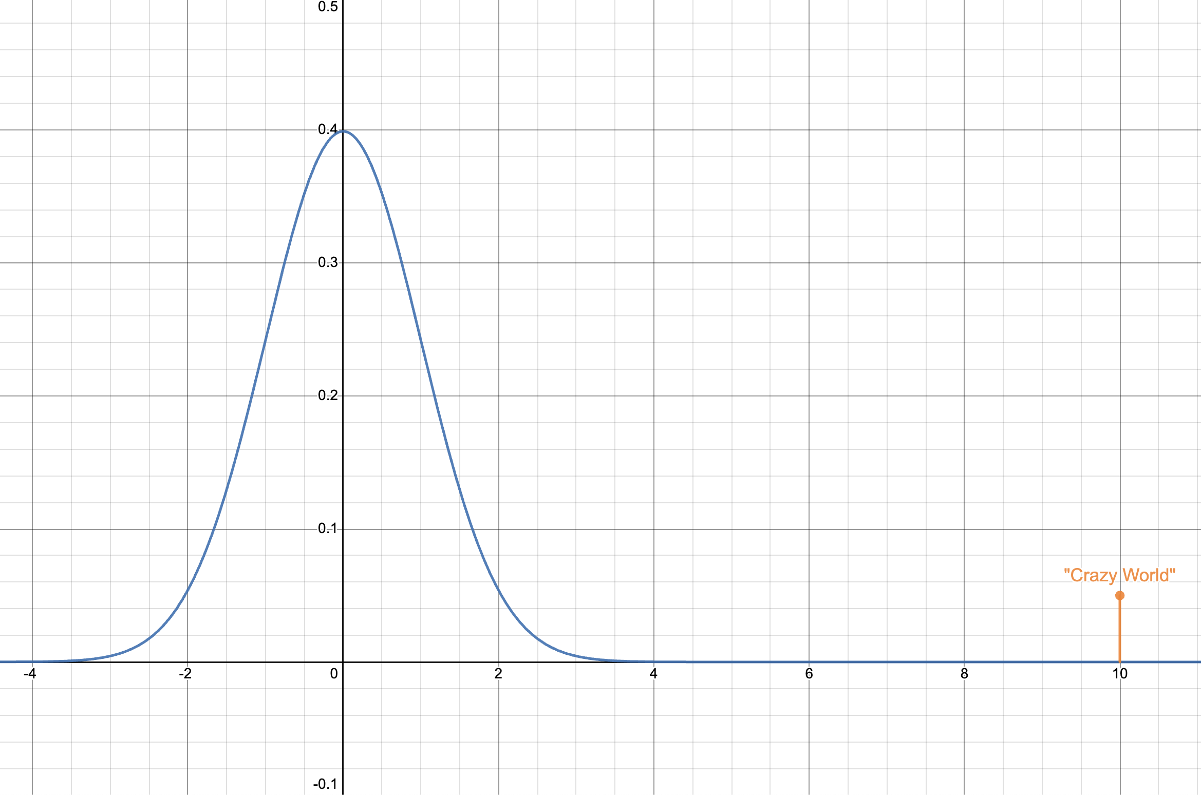
Suppose that in a “normal” world, we think an outcome is Normal(0, 1), but there’s a 5% chance that we’re in a “crazy world” where the outcome is 10. What should our overall 80% CI be?

We start with a rough estimate of our confidence interval in the combined world (normal+crazy). We approximate the quantiles of our mixture distribution as follows:

• In the “normal world”, our lower and upper bounds would be the 10th to 90th quantile of Normal(0,1), respectively
• In combined world, our interval should be higher. So, heuristically, we should take the 10th to 95th quantile of Normal(0,1) instead, because 5% of the right tail of the mixed distribution is already taken by the “crazy” world

But we can get a better estimate by computing exactly the 10th and 90th quantiles of the mixture distribution.

• Our mixed distribution assigns 0.95 weight to the Normal(0, 1) distribution, and 0.05 weight to a point mass at 10.

• Denote as \(P_L\) and \(P_R\) the left and right bounds under our “normal world” distribution, respectively. \(P_L\) and \(P_R\) are the 10th and 90th quantiles of the Normal(0, 1).

• Denote as \(P_L^*\) and \(P_R^*\) the new left and right bounds under our mixed distribution, respectively. We find \(P_L^*\) and \(P_R^*\) by writing and solving linear equations for them.

• We want \(0.95 P_L^* = 0.1\) so that 10% of the probability mass is to the left of \(P_L^*\) under the mixture distribution.

• Solving for \(P_L^*\) yields \(P_L^* \approx 0.105\).

• We want \(0.95 P_R^* + 0.05 = 1-0.9\) so that 10% of the probability mass of our mixture distribution is to the right of \(P_R^*\).

• Solving for \(P_R^*\) yields \(P_R^* \approx 0.947\).

This implies that better bounds for our 80% confidence interval in the “crazy world” are the 10.5th to 94.7th quantiles of Normal(0, 1).

14.4.2 Example 2

Consider example 1 above, but instead of a 5% chance of the “crazy world,” there is a 20% chance of the “crazy world.”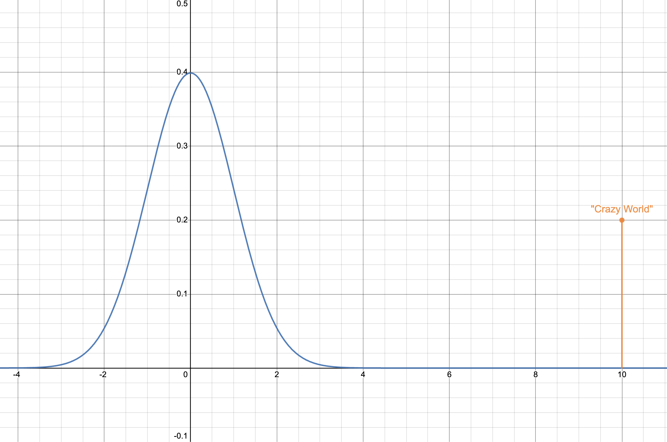

Following the steps from above, we would find ourselves with a nonsensical value for \(P_R^*\), trying to solve \(0.8 P_R^* + 0.2 = 0.1\) since we would get that \(P_R^* = -0.125\), but probabilities can not be negative.

The approach we took above breaks down because the quantile of our mixture distribution does not lie in the normal distribution of our “normal world,” but rather in the point mass of the “crazy world.”

Instead, we should observe that the 90th quantile for our mixture distribution actually lies within the point mass of the “crazy world,” so we must take 10 as our right bound.

14.4.3 General Method

Generalizing the approaches from the previous examples, we can obtain the desired quantiles of our mixture distribution by following these steps (these work when the distributions being mixed overlap only negligibly.)

• Determine which distribution the quantile of interest lies in.

• Write down and solve a linear equation based on the quantile of that distribution.

14.5 Summary

In this section, we explored to formal methods for combining uncertainties:

• Simulation (Squiggle)
• Graphical method (compute quantiles)

Running the simulation is easier and more straightforward, but graphical method is useful for building intuition (and can be done by hand!)