Regression to the mean is the idea that the top performers in one round generally do worse in the next round. Consider the following model for performance:
In any given round, the top performers have both luck and skill. But in the next round, they will likely have less luck.
One example of regression to the mean is heights of children. The scatterplot of adult children’s heights vs. the height of their father shows positive yet imperfect correlation. In other words, for a given number of standard deviations above the mean for the height of the father, we expect that the height of the child will be fewer standard deviations above the mean. Similarly, for a given number of standard deviations below the mean for the height of the father, we expect that the height of the child will be fewer standard deviations below the mean.
Some other examples of regression to the mean include:
CEOs who receive a high-profile award often “underperform expectations” in subsequent quarters
21.1.1 Accounting to Regression to the Mean
To account for regression to the mean, it is suggested to use long-run averages and to consider all candidates, not just previous top scorers (recall the “Other” option). Using long run averages can help average out the luck factor mentioned above.
21.1.1.1 Bayesian Interpretation for Regression to the Mean
Another way to account for regression to the mean is to adjust using a Bayesian prior. Recall our model that \(\text{performance} = X = X_{\text{skill}} + X_{\text{luck}}\). Suppose we have a first observation, \[X^{(1)} = X_{\text{skill}} + X_{\text{luck}}^{(1)}\] and we want to say something about what \(X^{(2)}\) will be. What we really want is \(\mathbb{P}(X_{\text{skill}} \mid X^{(1)})\). This requires a prior on \(X_{\text{skill}}\) and a distribution on \(X_{\text{luck}}\). For simplicity, suppose \[X_{\text{skill}} \sim \mathcal{N}(0, \sigma_{\text{skill}}^2)\]\[X_{\text{luck}} \sim \mathcal{N}(0, \sigma_{\text{luck}}^2)\] and we observe \(X^{(1)} = s\). Then, our conditional expectation for \(X_{\text{skill}} \mid X^{(1)} = s\) is \[\mathbb{E}[X_{\text{skill}} \mid X^{(1)} = s] = s \cdot \frac{\sigma_{\text{skill}}^2}{\sigma_{\text{skill}}^2 + \sigma_{\text{luck}}^2}\]
Interpreting this quantity, we can think of \(\frac{\sigma_{\text{skill}}^2}{\sigma_{\text{skill}}^2 + \sigma_{\text{luck}}^2}\) as the factor by which performance will regress to the mean. Observe that the wider the distribution of skills (higher \(\sigma_{skill}^2\)), the closer this factor is to one (luck plays less of a role, so there is less regression to the mean). Alternatively, the tighter the distribution of skills (lower \(\sigma_{skill}^2\)), the closer this factor is to zero (luck plays more of a role, so there is more regression to the mean).
Note that this is the same as the conditional expectation for \(X^{(2)} \mid X^{(1)}=s\) since \(X_{\text{luck}}\) has mean 0.
21.1.2 Selection of the Range
Consider the following example: suppose there is a certain city with five soccer leagues of different skill levels. Assume there was a Soccer Asseessment Test that measured the speed, coordination, strength, and soccer experience for players in that city.
Exercise
Think: Which of the following best describes how much the Soccer Assessment Test will correlate with a player’s success (measured by e.g. goals scored), within a league?
strongly negative correlation
moderately negative correlation
slight negative correlation
no correlation
slight positive correlation
moderate positive correlation
strong positive correlation
(whitespace to avoid spoilers)
(more whitespace to avoid spoilers)
One should expect slight correlation. Since the leagues already stratify players by skill level, we should expect that players that compete against each other are roughly the same skill level.
Exercise
Think: Now suppose that players were shuffled randomly among the leagues. Which of the following best describes how much the Soccer Assessment Test will correlate with a player’s success?
strongly negative correlation
moderately negative correlation
slight negative correlation
no correlation
slight positive correlation
moderate positive correlation
strong positive correlation
(whitespace to avoid spoilers)
One should expect moderate correlation. Since the players were shuffled across leagues, each team likely has a few high skill level players mixed with some medium and low skill level players. The players originally coming from the top leagues would probably have higher Soccer Assessment Test scores and almost certainly score more goals too.
21.2 L-Shaped Selection
Thought Experiment
Which of the following do you expect to be positive/negatively/uncorrelated?
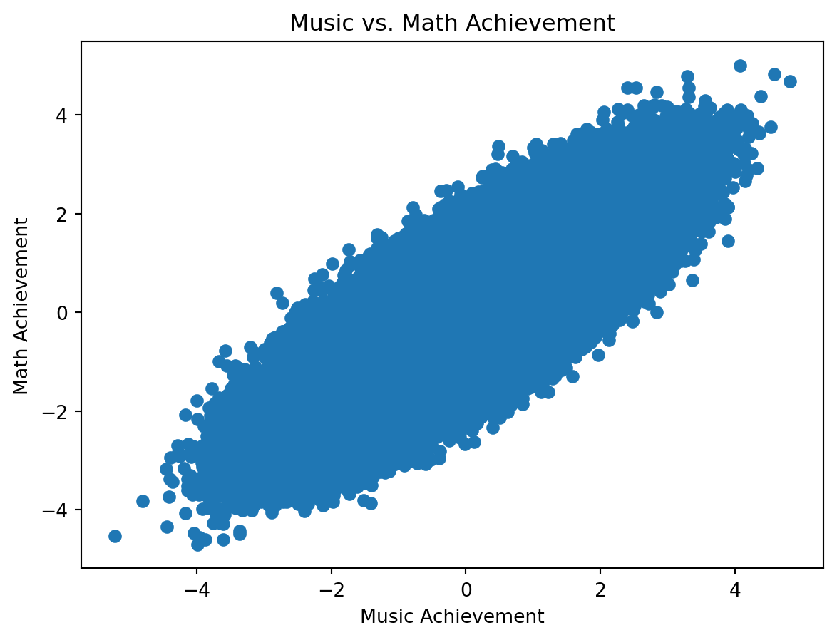
Some studies suggest that music and math achievement are positively correlated 1. This may come as a surprise, since you might find that among Berkeley students, students that are better at math tend to be worse at music, for example. However, we can make sense of this in the following way: suppose that in order to be admitted to Berkeley, one needs the sum of their math and music abilities to be above a certain threshold. Then, naturally, those that are good at math need not be as good at music and vice versa. This is called a “selection effect.”
Code
import matplotlib.pyplot as pltimport numpy as npnp.random.seed(165265)means = np.zeros(2)corr =0.8num_samples =1000000cov_matrix = np.array([[1, corr], [corr, 1]])music_and_math = np.random.multivariate_normal(means, cov_matrix, size=num_samples)print(music_and_math)plt.scatter(music_and_math[:, 0], music_and_math[:, 1]);plt.title("Music vs. Math Achievement");plt.xlabel("Music Achievement");plt.ylabel("Math Achievement");
thresh =6music_and_math_admitted_to_berkeley = music_and_math[np.sum(music_and_math, axis=1) > thresh]plt.scatter(music_and_math_admitted_to_berkeley[:, 0], music_and_math_admitted_to_berkeley[:, 1]);plt.title("Music vs. Math Achievement, Given Admission to Berkeley");plt.xlabel("Music Achievement")plt.ylabel("Math Achievement");
Notice that although there may be a positive correlation overall, once we condition on being admitted to Berkeley, the correlation becomes negative.
Some studies suggest that the rest are positively correlated as well, though there is more controversy for those than for music and math achievement.↩︎